Design Project #1 (CMG)
System
The first project that you will complete this semester is to design, implement, and test a controller that uses a single-gimbal control moment gyroscope (CMG) to reorient a platform in a gravitational field, as pictured below:
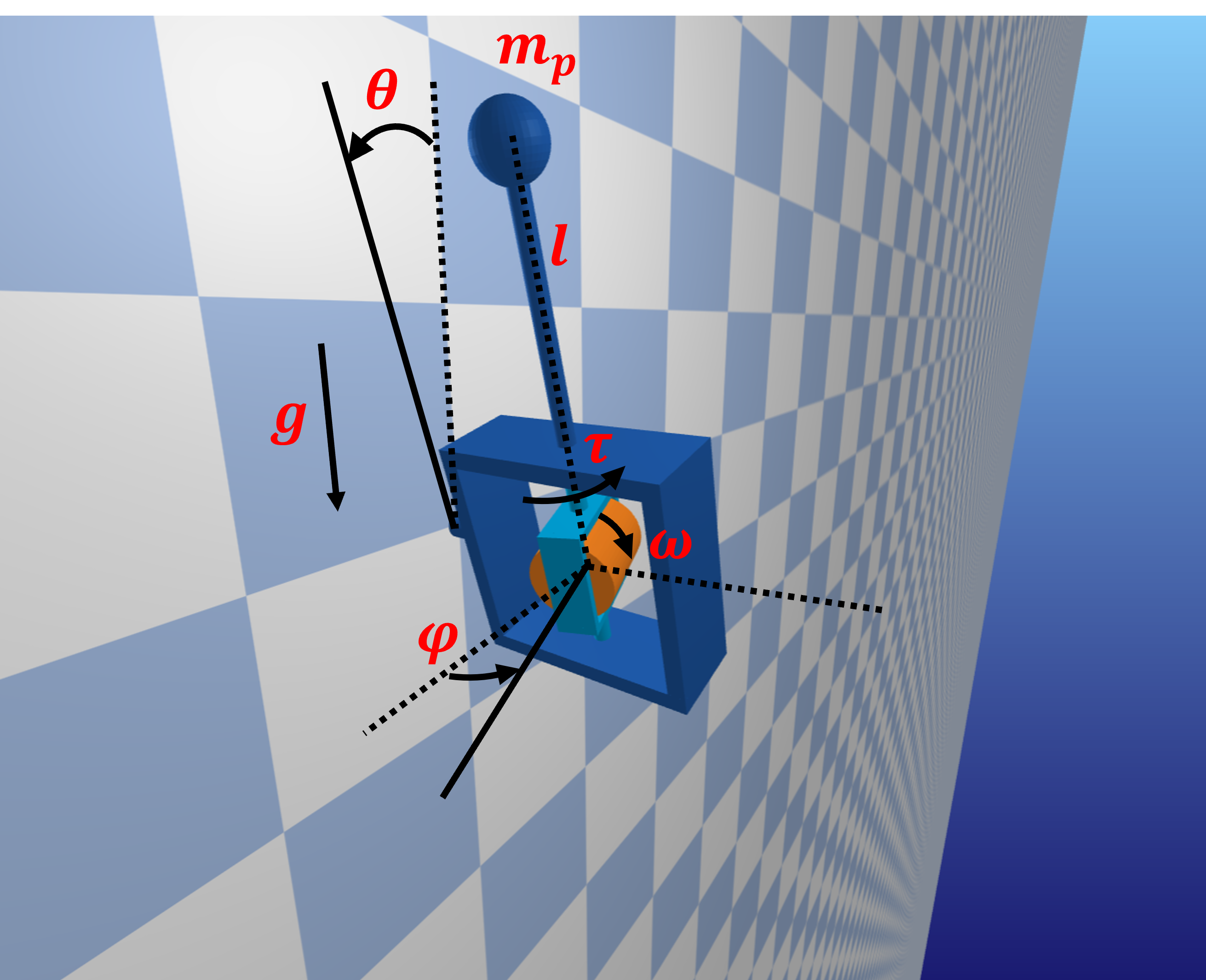
This system has three parts:
- A frame or platform (dark blue) that can rotate freely about its platform through an angle \(\theta\). Think of this as a spacecraft that is confined to rotate about its pitch axis, as if it were being tested on the ground.
- A gimbal (light blue) that can be driven by a motor to rotate about a perpendicular axis with respect to the frame with an angle \(\phi\).
- A rotor (orange) that can be driven by a motor to spin about yet another perpendicular axis with respect to the gimbal.
The input to the system is some torque \(\tau\) that is applied to the gimbal causing it to rotate through an angle \(\phi\). Gravity \(g\) is acting directly downwards. Whereas it is not intuitive, we will find that this torque can result in changes to both \(\phi\) and, through the conservation of momentum, \(\theta\).
In simpler terms, if the rotor is spun at a high rate, then an “input torque” applied to the gimbal will, through conservation of angular momentum, result in an “output torque” applied to the platform. This output torque can be used, in particular, to change the orientation of the platform.
Context
Reaction wheels and control-moment gyroscopes (CMGs) are two different non-propulsive actuators (i.e., actuators that do not consume fuel) that are commonly used to control the attitude of spacecraft.
A reaction wheel spins at a variable rate about an axis that is fixed with respect to the spacecraft. If the spacecraft applies a torque to this wheel with a motor (either speeding it up or slowing it down), then an equal and opposite torque is applied to the spacecraft.
A single-gimbal CMG also has a spinning wheel, but with two key differences: (1) the wheel spins at a constant rate instead of at a variable rate, and (2) the wheel is held by a gimbal that allows the axis of spin to be tilted with respect to the spaceraft instead of staying fixed.
In particular, if the wheel in a single-gimbal CMG — often called a rotor — is spun at a high rate, then an “input torque” applied to the gimbal will, through conservation of angular momentum, result in an “output torque” applied to the platform about an axis perpendicular both to the gimbal axis and the rotor axis.
One advantage of using a single-gimbal CMG over a reaction wheel is that this output torque can be much higher than the input torque — a so-called “torque amplification” effect. That is to say, CMGs have the ability to generate large torques with relatively low power consumption. This makes them well-suited for long-duration space missions — including geosynchronous satellites and interplanetary probes — where power and weight constraints are significant considerations. This also means that CMGs can, in general, produce much larger torques than reaction wheels, which can be useful for attitude control of very large spacecraft. The International Space Station (ISS) is one example of a large spacecraft whose attitude is controlled by CMGs — here is an image of a CMG being installed on ISS by an STS-118 crew member: 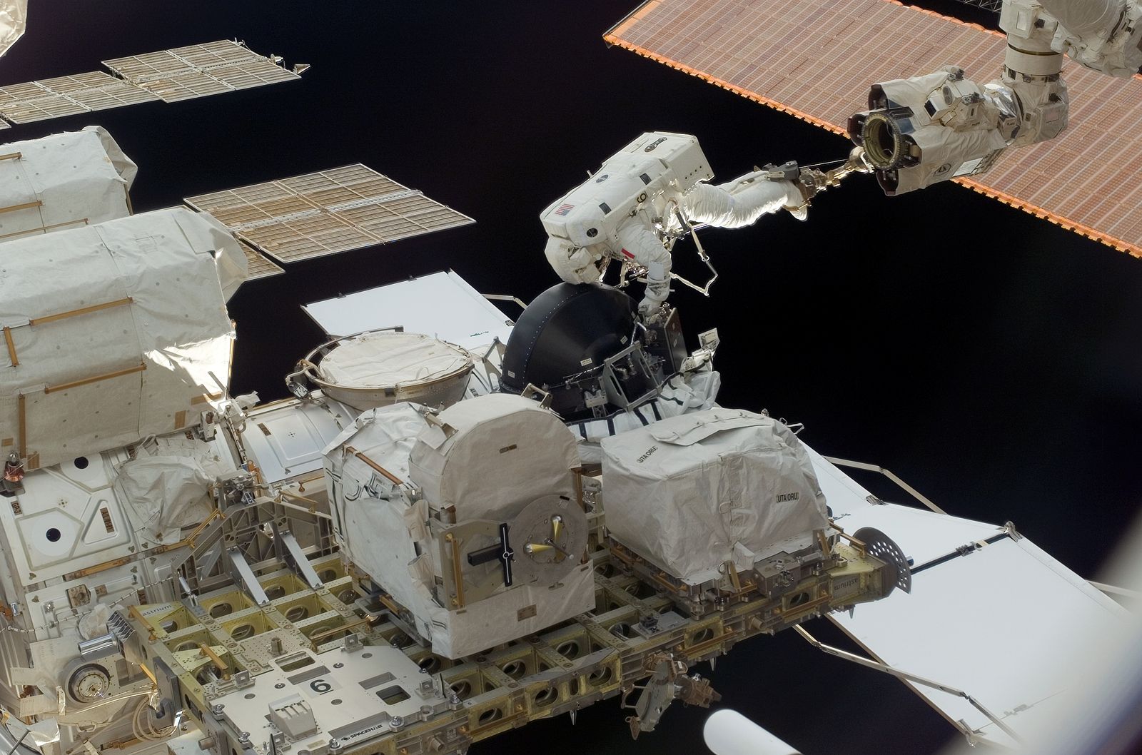
ISS uses four double-gimbal CMGs rather than the one single-gimbal CMG you will be considering in this project, although the principles of operation are similar. These CMGs have a life expectency of about 10 years, contain a rotor that spins at 691 rad/s (6600 rpm), and can produce an output torque of 258 N-m (190 ft-lbf). The orientation of ISS can be fine-tuned to point exactly at a target By controlling the tilt of each CMG.
There are disadvantages to using CMGs instead of reaction wheels, of course. One disadvantage, for example, is that the dynamics of a CMG are more complicated than those of a reaction wheel and require a more sophisticated controller.
This first design project will familiarize you with the operational concepts and physics behind the use of CMGs on modern spacecraft, and in particular will give you a sense of what it takes to control them.
You can read more about CMGs and their use for spacecraft attitude control in Fundamentals of Spacecraft Attitude Determination and Control (Markley and Crassidis, 2014).
Model
The first step we will take will be to derive the equations of motion of the system. As usual, the first step in the Lagrangian mechanics approach is to calculate the total kinetic energy of the system and the total potential energy of the system with respect to the generalized coordinates and their derivatives. Then, we calculate the Lagrangian of the system:
\[L=T-V,\]where \(T\) is the total kinetic energy of the system and \(V\) is the total potential energy of the system.
Do this, we get
\[L=0.005\sin^{2}(\phi)\dot{\phi}^{2}-4\sin(\phi)\dot{\theta}-7.36\cos(\theta)+0.0015\dot{\phi}^{2} + 0.578\dot{\theta}^{2}+200\]Finally, we can get the equations of motion via the formula:
\[\frac{\partial}{\partial t} \left( \frac{\partial L}{\partial \dot{\theta}} \right) - \frac{\partial L}{\partial \theta} = 0,\] \[\frac{\partial}{\partial t} \left( \frac{\partial L}{\partial \dot{\phi}} \right) - \frac{\partial L}{\partial \phi} - \tau = 0.\]Solving, we find:
\[0.01\sin^{2}({\phi})\ddot{\theta}+0.02\sin({\phi})\cos({\phi})\dot{\phi}\dot{\theta} - 7.36\sin({\theta}) - 4\cos({\phi})\dot{\phi}+1.16\ddot{\theta} = 0\] \[-\tau -0.01\sin({\phi})\cos({\phi})\dot{\theta}^{2}+4\cos({\phi})\dot{\theta}+0.03\ddot{\phi}=0.\]You are provided with the following:
ae353_cmg-Template.ipynb– A Jupyter notebook that provides a demo of the interface to the CMG simulator to help you get started. As a suggestion: make a copy of this notebook and work on the copy instead of the original template. This way, you can always refer back to the original template if needed. This is also the file that will contain your solution.ae353_cmg-EoM.ipynb– A Jupyter notebook that provides the derivation of equations of motion for the CMGae353_cmg.py– A Python script that provides an interface to pybullet simulator. This is imported in the Jupyter notebook as shown in ae353_cmg-EoM.ipynb. Do not modify this filecmg_vis– A folder containing files needed for the simulator. You don’t need to modify any of the files in this subfolder for the project
ae353_cmg.py and the files in the urdf subfolder are needed for the simulator to run and hence should always be in the same folder as the one in which the notebook you are working on is. However, you do not have to directly access or modify any of these files for this project.
The system starts at whatever initial conditions you choose. The goal is to bring the platform back to rest at some desired angle that you get to choose. Careful! Not all platform angles may be achievable.
Your tasks
Please do the following things:
- Choose a platform angle that you want to achieve (you will likely find that there are exactly two choices).
- Linearize the model about an equilibrium point that corresponds to this platform angle and express the result in state-space form.
- Design a linear state feedback controller and verify that the closed-loop system is asymptotically stable in theory. Note that here you verify the asymptotic stability with your controller on the linearized model of the system.
- Implement this controller and verify that the closed-loop system is asymptotically stable in simulation, at least when initial conditions are close to equilibrium. Note that here you are applying the linear state feedback controller you designed to the original nonlinear model of the system given in the simulation.
Remember that your controller is not expected to “work” in all cases and that you should try hard to establish limits of performance (i.e., to break your controller).
For example, it is insufficient to simulate the application of your controller from one set of initial conditions, plot the resulting trajectory, argue that this trajectory is consistent with the closed-loop system being stable, and conclude (wrongly) that your controller “works.” Instead, you should test your controller from many different sets of initial conditions and should try to distinguish between conditions that do and do not lead to failure.
More generally, please focus on generating results that could be used to support a comprehensive argument for or against the use of single-gimbal CMGs in a future space mission.
Then, consider at least one of the following questions:
- Is there a difference between the trajectory that is predicted by your linear model and the one that results from the nonlinear simulation?
- How do the initial conditions affect the resulting motion?
- How does the choice of goal angle affect the resulting motion?
In addition to above, you are also welcome to consider a similar question that you come up with on your own. Genuine efforts on performing extra work and gaining further insight into control of this system may attract bonus credits.
Explicitly write down the solutions to the above posed questions. For example, consider the question: Linearize the system about an equilibrium point and express the result in state-space form. You are expected to explicitly write down the matrices A, B, C, D (whichever is applicable in this scenario). Additionally, simply mentioning an equilibrium point is not sufficient – reason it out mathematically or in words.
Bonus points: There are many ways to go beyond minimum requirements (what happens if you change the boom mass \(m\)? what happens if you change the rotor velocity \(v_\text{rotor}\)? is it possible to swing the platform from its “down” configuration to its “up” configuration?) — come talk to us if you want an extra challenge.
Your deliverables
We will use Canvas for submitting design projects. You must create a compressed folder (.zip) titled DP1-submission with the code and the report in the format described below and submit by September 22, 11:59pm
Code
This code will satisfy the following requirements:
- It must be in a folder called code (lower case).
- It must include a single notebook called
GenerateResults.ipynbthat could be used to reproduce all of the results that you show in the report. (You can work in the ae353_cmg-Template.ipynb notebook (or the copy that you created) and then rename it toGenerateResults.ipynbwhen you are ready to submit.) - It must include all the other files (with the right folder structure) that are necessary for
GenerateResults.ipynbto function. - It must not rely on any dependencies other than those associated with the conda environment.
Report
This report will satisfy the following requirements:
- It must be a single PDF document that is called
report.pdfand that conforms to the guidelines for Preparation of Papers for AIAA Technical Conferences. In particular, you must use the LaTeX manuscript template. - It must have a descriptive title, name of the author, an abstract, and a list of nomen- clature.
- It must say how you addressed all of the required tasks (see above).
- It must tell a story that shows you have found and explored something that interests you.
- It must acknowledge and cite any sources.
- It should preferably be about 5 pages in length — it will be hard to show off your work with anything shorter, and it will be hard to keep readers’ attention with anything longer. You may never have used LaTeX before. Don’t be afraid! Help will be provided, and you will learn a lot. You will submit the PDF document produced using LaTeX. In particular, we recommend using Overleaf, an easy to use web-based LaTeX editor.
You may organize your report however you like, but a natural structure might be to have sections titled Introduction, Model, Design, Results, and Conclusion.
Submission Instructions
To make it easier logistically, there will be two assigned submissions for this project on Canvas. Please submit the following separately:
- Report: Submit a pdf version of your report.
- Code: Compress your code into a zip file and submit the zip file. Before compressing your files into a compressed zip file for submission, the project folder should look like this:
├── ae353_cmg-EoM.ipynb
├── ae353_cmg-Intro.ipynb
├── GenerateResults.ipynb # this is your solution file
├── ae353_cmg.py
└── cmg_vis
    ├── check.png
    ├── cmg.png
    ├── cmg.pptx
    ├── cmg.urdf
    ├── concrete.png
    ├── cube.stl
    ├── cylinder.stl
    ├── plane.urdf
    ├── plane_big.obj
    └── sphere.stl
Evaluation
Your work will be evaluated based on:
- (60%) Completion of the requirements and the resulting description of the results (60%)
- (25%) Submission of working code
- (15%) Your report being formatted correctly
Late submission will be penalized (by up to 25% for the first week of delay—prorated for the actual amount of delay—and 50% after then), but extraordinary efforts may receive extra commendation. The focus of our evaluation of your report this time (as you learn how to use LaTeX) will be on content—we will not look at style, grammar, or any other aspect of your presentation, as long as there is no barrier to understanding your work.
Frequently asked questions
How do I get started?
The first thing you should do is update your local copy of the repository with the DesignProblem01 file, to do this, please follow the installation instructions, very specifically, follow the ‘Do this every time’ section and run the command after navigating to the directory where you have cloned the repository:
conda activate ae353
git pull
This will update your local copy of the repository with the code for Design Problem 01.
Verify that you can run the simulation in the ae353_cmg-Template.ipynb notebook, and mess around a little bit with different actuator commands (e.g., constant torques applied to the gimbal and the rotor) to get a sense for how the system responds. After that, if you have read the entire project description and are not sure how to proceed, then take your best guess and ask a question on Canvas or attend in-person discussion sessions dedicated for design projects. Improving your ability to get unstuck by asking a good question is an explicit goal of this course.
What is “the model” that I should linearize?
The standard way to produce a state space model is to linearize a set of ODEs that describe the equations of motion. You will find ODEs that describe the equations of motion for the CMG system in the system section above. If you are interested, the derivation of these ODEs has also been provided for you in the ae353_cmg-EoM.ipynb notebook. I would start with these ODEs.
You will quickly realize that it may be a good idea to restrict your attention only to the platform and the gimbal, treating the rotor as a source of torque. In particular, for the purpose of control design and analysis, you may want to assume that the angular velocity of the rotor is constant and to completely ignore the second-order ODE that describes how this rotor responds to applied torque. It is entirely up to you how to proceed, though. There is no one right answer.